Contents
- Introduction
- A Job Shop Simulation Application
- Job Shop Data Model
- Job Shop Implementation
- Conflict Analysis
Introduction
Models of systems can come in all sorts of shapes and sizes. The simplest sketch of a system on the back of a napkin is a model that can tell us something about the intended structure and behaviour of the system. Models tend to fall into distinct categories that reflect their intent. Models of usage (such as use-case models) try to capture the client view of the system, i.e. what does the system offer? Archtecture models try to capture the major components of the system and how they will communicate. Data models try to capture the information that the system processes. Dynamic models try to produce descriptions of how the system behaves under certain conditions. In all cases, these models may be constructed as lightweight sketches that ignore implementation detail or constructed as detailed blueprints including key implementation features.To be effective, modelling must be integrated with a project development method. There are many such methods; one significant method is to use modelling to produce a complete executable simulation of the system. The model is representative of the real system and is used to run test cases. The model does not need to deal with complex implementation details. Once the executable model has been developed and used to analyse the behaviour of the required system, it can be used as an executable blueprint for the real system.
There are a number of advantages to this approach: results can be produced in a short time; requirements engineering can involve presenting stakeholders with a simulation of the required system; the languages used for executable modelling support good debugging and instrumentation; the languages provide high level support for manipulating data and representing key application components; using the executable model as a blueprint significantly reduces the gap between design and implementation.
In order to simulate a system, a model must include the actions that the system performs. There are a variety of ways of modelling actions including state machines and model based action languages. Modelling actions falls broadly into two categories that differ depending on whether the model is to be executable or whether it is to be used to analyse system executions. The former allows the model to be run. The latter statically describes the properties of executions.
XOCL can be used to define both categories of dynamic model behaviour. XOCL supports operations that are added to model components in order to execute the modelled application. XOCL can be extended with constructs that suit the application domain and therefore make it easier to define the simulation, to analyse it and to translate it to a complete implementation.
This chapter shows how XOCL is used to produce a system simulation. Section specifies a simple job-shop application and shows how the simulator will behave. Section describes how the simulation is implemented. Finally, section describes how dynamic execution behaviours can be modelled and subsequently analysed.
To top.
A Job Shop Simulation Application
Scheduling jobs is a typical example of an application that can
benefit from simulation. There are many ways in which jobs can be
scheduled to machines that process the jobs and the behaviour of a
scheduling application can change depending on many different features
of the application. Opportunistic scheduling is a simple type of
scheduling whereby jobs are allocated to machines as soon as the
machine becomes available without any fancy analysis of the best use of
resources. This section describes an executable model for opportunistic
scheduling.
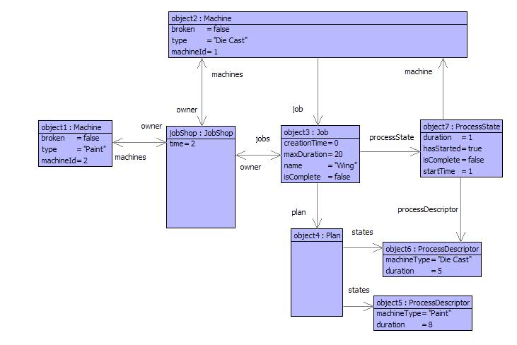
The figure below shows a simple jobs shop as a tree of components. The
job shop contains jobs that must be processed and machines that can
process the jobs. In this case the application is to process an
aircraft wing. The single job named Wing has a plan that specifies a
sequence of processes that must be performed in order. The wing must be
case by a die casting machine and then painted by a painting machine.
The job-shop has exactly one machine of each type (therefore the task
is do-able).

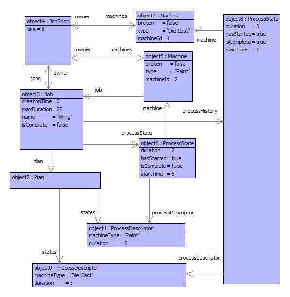
The figure below shows the steps in performing this simple
simulation. The initial state of the jobs shop shows that the Wing job
is not allocated to any machine. The job is then allocated to the Die
Case machine for 5 units of time after which is switches to the Paint
machine for 8 units of time and finally the job is complete and not
allocated to any machines.
 |
 |
 |
|
To top.
Job Shop Data Model
The figure below shows a model of a job-shop consisting of jobs to
be processed and machines that can process jobs. The required
application is an opportunistic scheduler that will allocate jobs to
appropriate machines as soon as they become available. Each job has a
plan that is a sequence of process descriptors: at any given time, a
job is either completed or is waiting to be allocated to a machine or
is being processed by a machine. A machine performs processes of a
given type and can only process one job at a time.

The model allows various configurations of machines and jobs to be
created. By attaching actions to the classes in the model it is then
possible to simulate the execution of the configuration. The results of
the simulation can be used to analyse both the configuration and the
impact of modifications to the configuration. These include:
determining the overall execution time, whether there are any
bottlenecks in the system; the effect of adding and removing machines
of various types; and, the amount of time machines are left idle.
Here are key features of the model:
- Class JobShop records the current time and has a number of jobs and machines. At the end of the simulation, all of the jobs are complete. Each machine has a unique id, a type and may be broken. The type of the machine determines the tasks that it can perform. A machine has a current job that may be empty. If it is non-empty then the machine is currently processing the job and the type of the machine must match the process at the head of the job's plan.
- Class Job has a name, a creation time (allowing for jobs to be dynamically added to the system) and a maximum allowed duration (allowing for the simulation to determine whether a job is taking too long). A job becomes complete when the last process in its plan is performed by a machine.
- Each job has a plan consisting of a sequence of process descriptors. Class ProcessDescriptor defines the machine that must perform the processing and the length of time that the process takes.
- A job is in a current state, which may be null if it is between tasks. If the job is being processed by a machine then the current state has a process descriptor and a machine: the type of the machine must match the type in the prcess descriptor.
- class ProcessState records the time at which it is created. It knows the duration that the task must take from the process descriptor and can therefore describe when it is complete. When a task is complete, the current state of a job is set to null, however the job has a process history that can be used for analysis (in a real implementation a job may not require a process history). The process history is the sequence of all process states that the job has performed.
The figure below shows a simple initial state for a job shop that processes aircraft wings. The job is started with an initial process state set up for the initial process descriptor in the plan; however, the process state shows that the process has not started and is not yet allocated to a machine.

A trace of the simulation is shown below:
[1] XMF> ProcessWing::jobShop.run();
[1  ] Job Wing becomes scheduled at machine Die Cast:1.
[2  ] Machine Die Cast:1 processing job Wing (1 of 5 units)
[3  ] Machine Die Cast:1 processing job Wing (2 of 5 units)
[4  ] Machine Die Cast:1 processing job Wing (3 of 5 units)
[5  ] Machine Die Cast:1 processing job Wing (4 of 5 units)
[6  ] Machine Die Cast:1 completes job Wing.
[6  ] Job Wing becomes scheduled at machine Paint:2.
[7  ] Machine Paint:2 processing job Wing (1 of 8 units)
[8  ] Machine Paint:2 processing job Wing (2 of 8 units)
[9  ] Machine Paint:2 processing job Wing (3 of 8 units)
[10 ] Machine Paint:2 processing job Wing (4 of 8 units)
[11 ] Machine Paint:2 processing job Wing (5 of 8 units)
[12 ] Machine Paint:2 processing job Wing (6 of 8 units)
[13 ] Machine Paint:2 processing job Wing (7 of 8 units)
[14 ] Machine Paint:2 completes job Wing.
true
[1] XMF>
[1] XMF> ProcessWing::jobShop.idleTimes();
Machine Paint:2 was idle at time 1.
Machine Paint:2 was idle at time 2.
Machine Paint:2 was idle at time 3.
Machine Paint:2 was idle at time 4.
Machine Paint:2 was idle at time 5.
Machine Die Cast:1 was idle at time 7.
Machine Die Cast:1 was idle at time 8.
Machine Die Cast:1 was idle at time 9.
Machine Die Cast:1 was idle at time 10.
Machine Die Cast:1 was idle at time 11.
Machine Die Cast:1 was idle at time 12.
Machine Die Cast:1 was idle at time 13.
true
[1] XMF>
[1] XMF> ProcessAircraft::jobShop.run();To top.
[1 ] Job Wing1 becomes scheduled at machine Die Cast:3.
[2 ] Machine Die Cast:3 processing job Wing1 (1 of 5 units)
[3 ] Machine Die Cast:3 processing job Wing1 (2 of 5 units)
[4 ] Machine Die Cast:3 processing job Wing1 (3 of 5 units)
[5 ] Machine Die Cast:3 processing job Wing1 (4 of 5 units)
[6 ] Machine Die Cast:3 completes job Wing1.
[6 ] Job Wing1 becomes scheduled at machine Paint:4.
[7 ] Job Tail1 becomes scheduled at machine Die Cast:3.
[7 ] Machine Paint:4 processing job Wing1 (1 of 8 units)
[8 ] Machine Die Cast:3 processing job Tail1 (1 of 5 units)
[8 ] Machine Paint:4 processing job Wing1 (2 of 8 units)
[9 ] Machine Die Cast:3 processing job Tail1 (2 of 5 units)
[9 ] Machine Paint:4 processing job Wing1 (3 of 8 units)
[10 ] Machine Die Cast:3 processing job Tail1 (3 of 5 units)
[10 ] Machine Paint:4 processing job Wing1 (4 of 8 units)
[11 ] Machine Die Cast:3 processing job Tail1 (4 of 5 units)
[11 ] Machine Paint:4 processing job Wing1 (5 of 8 units)
[12 ] Machine Die Cast:3 completes job Tail1.
[12 ] Machine Paint:4 processing job Wing1 (6 of 8 units)
[13 ] Job Tail1 becomes scheduled at machine Paint:2.
[13 ] Job Tail2 becomes scheduled at machine Die Cast:3.
[13 ] Machine Paint:4 processing job Wing1 (7 of 8 units)
[14 ] Machine Paint:2 processing job Tail1 (1 of 8 units)
[14 ] Machine Die Cast:3 processing job Tail2 (1 of 5 units)
[14 ] Machine Paint:4 completes job Wing1.
[14 ] Job Wing1 becomes scheduled at machine Assemble:6.
[15 ] Machine Paint:2 processing job Tail1 (2 of 8 units)
[15 ] Machine Die Cast:3 processing job Tail2 (2 of 5 units)
[15 ] Machine Assemble:6 processing job Wing1 (1 of 3 units)
[16 ] Machine Paint:2 processing job Tail1 (3 of 8 units)
[16 ] Machine Die Cast:3 processing job Tail2 (3 of 5 units)
[16 ] Machine Assemble:6 processing job Wing1 (2 of 3 units)
[17 ] Machine Paint:2 processing job Tail1 (4 of 8 units)
[17 ] Machine Die Cast:3 processing job Tail2 (4 of 5 units)
[17 ] Machine Assemble:6 completes job Wing1.
[18 ] Machine Paint:2 processing job Tail1 (5 of 8 units)
[18 ] Machine Die Cast:3 completes job Tail2.
[18 ] Job Tail2 becomes scheduled at machine Paint:4.
[19 ] Machine Paint:2 processing job Tail1 (6 of 8 units)
[19 ] Job Nose becomes scheduled at machine Die Cast:3.
[19 ] Machine Paint:4 processing job Tail2 (1 of 8 units)
[20 ] Machine Paint:2 processing job Tail1 (7 of 8 units)
[20 ] Machine Die Cast:3 processing job Nose (1 of 5 units)
[20 ] Machine Paint:4 processing job Tail2 (2 of 8 units)
[21 ] Machine Paint:2 completes job Tail1.
[21 ] Machine Die Cast:3 processing job Nose (2 of 5 units)
[21 ] Machine Paint:4 processing job Tail2 (3 of 8 units)
[21 ] Job Tail1 becomes scheduled at machine Assemble:6.
[22 ] Machine Die Cast:3 processing job Nose (3 of 5 units)
[22 ] Machine Paint:4 processing job Tail2 (4 of 8 units)
[22 ] Machine Assemble:6 processing job Tail1 (1 of 3 units)
[23 ] Machine Die Cast:3 processing job Nose (4 of 5 units)
[23 ] Machine Paint:4 processing job Tail2 (5 of 8 units)
[23 ] Machine Assemble:6 processing job Tail1 (2 of 3 units)
[24 ] Machine Die Cast:3 completes job Nose.
[24 ] Machine Paint:4 processing job Tail2 (6 of 8 units)
[24 ] Machine Assemble:6 completes job Tail1.
[25 ] Job Nose becomes scheduled at machine Paint:2.
[25 ] Machine Paint:4 processing job Tail2 (7 of 8 units)
[26 ] Machine Paint:2 processing job Nose (1 of 8 units)
[26 ] Machine Paint:4 completes job Tail2.
[26 ] Job Tail2 becomes scheduled at machine Assemble:6.
[27 ] Machine Paint:2 processing job Nose (2 of 8 units)
[27 ] Machine Assemble:6 processing job Tail2 (1 of 3 units)
[28 ] Machine Paint:2 processing job Nose (3 of 8 units)
[28 ] Machine Assemble:6 processing job Tail2 (2 of 3 units)
[29 ] Machine Paint:2 processing job Nose (4 of 8 units)
[29 ] Machine Assemble:6 completes job Tail2.
[30 ] Machine Paint:2 processing job Nose (5 of 8 units)
[31 ] Machine Paint:2 processing job Nose (6 of 8 units)
[32 ] Machine Paint:2 processing job Nose (7 of 8 units)
[33 ] Machine Paint:2 completes job Nose.
[33 ] Job Nose becomes scheduled at machine Assemble:6.
[34 ] Machine Assemble:6 processing job Nose (1 of 3 units)
[35 ] Machine Assemble:6 processing job Nose (2 of 3 units)
[36 ] Machine Assemble:6 completes job Nose.
true
Job Shop Implementation
The previous section has specified a job shop scheduling simulation in terms of a general model consisting of jobs, plans and machines. Non-executable modelling would have to stop at this point: the execution would be left implicit, perhaps specified as pre and post-conditions on various model operations. Executable modelling allows the models to be brought to life in terms of simulation. Depending on the application requirements, it is possible for the executable model to be the application, however that is not the issue here. This section describes the implementation of the key features of the simulation by defining operations on the classes defined in figure .A job shop simulation is initiated by the run operation:
context JobShop
  @Operation runJobs()
    @While not jobs->forAll(job | job.isComplete()) do
      self.time := time + 1
      @For machine in machines do
        machine.process(self)
      end
    end
  end
context Machine
  @Operation process(jobShop:JobShop)
    if not broken
    then
      if job <> null
      then self.processJob(jobShop)
      else self.findJob(jobShop)
      end
    else format(stdout,"~S:~S is broken at the moment.",Seq{type,machineId})
    end
  end
context Machine
  @Operation processJob(jobShop:JobShop)
    job.tick();
    if job.isComplete()
    then
      self.printCompleted(jobShop.time(),job);
      self.setJob(null)
    else self.printProcessing(jobShop.time(),job)
    end
  end
context Machine
  @Operation findJob(jobShop)
    @Find(job,jobShop.jobs())
      when
        not job.processState().hasStarted() andthen
        job.processState().processDescriptor().machineType = type
      do self.setJob(job);
         job.processState().start(jobShop.time(),self);
         self.printJobScheduled(jobShop.time(),job)
    end
  end

context ProcessState
  @Operation start(time:Integer,machine:Machine)
    self.setHasStarted(true);
    self.setStartTime(time);
    self.setMachine(machine)
  end
context Job
  @Operation tick()
    processState.tick();
    if processState.isComplete()
    then self.nextProcessState()
    end
  end

context ProcessState
  @Operation tick()
    if hasStarted and not isComplete
    then
      self.setDuration(duration + 1);
      if duration >= processDescriptor.duration()
      then self.setIsComplete(true)
      end
    end
  end
context Job
  @Operation nextProcessState()
    self.addToProcessHistory(processState);
    self.setProcessState(plan.nextProcessState(processState));
    if processState = null
    then self.setIsComplete(true)
    end
  end

context Plan
  @Operation nextProcessState(current:ProcessState):ProcessState
    let index = states->indexOf(current.processDescriptor())
    in if index + 1 >= states->size
       then null
       else
         let next = states->at(index + 1)
         in ProcessState(next)
         end
       end
    end
  end
context JobShop
  @Operation idleTimes()
    @Count t from 1 to time do
      @For machine in machines do
        if not jobs->exists(job | job.processedBy(machine,t))
        then self.printIdle(machine,t)
        end
      end
    end
  end

context Job
  @Operation processedBy(machine,time):Boolean
    processHistory->exists(state |
      state.machine() = machine and
      state.startTime() <= time and
      (state.startTime() + state.duration()) >= time)
  end
context JobShopTo top.
@Operation lateJobs():Set(Job)
jobs->select(job | job.maxDuration() < job.duration())
end
context Job
@Operation duration():Integer
let state = processHistory->last
in (state.startTime() + state.duration()) - creationTime
end
end
Conflict Analysis
An interesting analysis dertmines whether or not there are two jobs
that ever require the same machine at the same time. This analysis
requires a slightly diffferent type of simulation from that described
so far. In order to determine whether there may be a conflict, the job
shop is symbolically executed, creating histories of possible
allocations of jobs to machines. These allocations can then be analysed
to determine whether any of them overlap.Given the initial state of the job-shop it is possible to calculate the scheduling options by analysing the plan for each job and allocating the job to the machines it requires. The result of doing this for each job is a collection of possible histories for the simulation. An execution of the simulation is represented by one possible history for each of the jobs. If there is a machine that is required by two different jobs in all possible histories then it is not possible to optimally schedule the jobs, i.e. there is a bottleneck arising from a conflict.
Consider the ProcessAircraft example given in a previous section. Here are all the histories calculated for the jobs:
Histories calculated for job Wing1:
  Option:
     Machine 3 is used from 0 to 5
     Machine 4 is used from 5 to 13
     Machine 5 is used from 13 to 16
  Option:
     Machine 3 is used from 0 to 5
     Machine 4 is used from 5 to 13
     Machine 6 is used from 13 to 16
  Option:
     Machine 3 is used from 0 to 5
     Machine 2 is used from 5 to 13
     Machine 6 is used from 13 to 16
  Option:
     Machine 3 is used from 0 to 5
     Machine 2 is used from 5 to 13
     Machine 5 is used from 13 to 16
Histories calculated for job Tail1:
  Option:
     Machine 3 is used from 0 to 5
     Machine 4 is used from 5 to 13
     Machine 5 is used from 13 to 16
  Option:
     Machine 3 is used from 0 to 5
     Machine 4 is used from 5 to 13
     Machine 6 is used from 13 to 16
  Option:
     Machine 3 is used from 0 to 5
     Machine 2 is used from 5 to 13
     Machine 6 is used from 13 to 16
  Option:
     Machine 3 is used from 0 to 5
     Machine 2 is used from 5 to 13
     Machine 5 is used from 13 to 16
Histories calculated for job Tail2:
  Option:
     Machine 3 is used from 0 to 5
     Machine 4 is used from 5 to 13
     Machine 5 is used from 13 to 16
  Option:
     Machine 3 is used from 0 to 5
     Machine 4 is used from 5 to 13
     Machine 6 is used from 13 to 16
  Option:
     Machine 3 is used from 0 to 5
     Machine 2 is used from 5 to 13
     Machine 6 is used from 13 to 16
  Option:
     Machine 3 is used from 0 to 5
     Machine 2 is used from 5 to 13
     Machine 5 is used from 13 to 16
Histories calculated for job Nose:
  Option:
     Machine 3 is used from 0 to 5
     Machine 4 is used from 5 to 13
     Machine 5 is used from 13 to 16
  Option:
     Machine 3 is used from 0 to 5
     Machine 4 is used from 5 to 13
     Machine 6 is used from 13 to 16
  Option:
     Machine 3 is used from 0 to 5
     Machine 2 is used from 5 to 13
     Machine 6 is used from 13 to 16
  Option:
     Machine 3 is used from 0 to 5
     Machine 2 is used from 5 to 13
     Machine 5 is used from 13 to 16
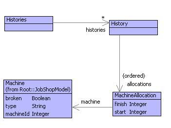
Each plan produces n instance of Histories:
context Plan
  @Operation histories(jobShop)
    let h = Histories()
    in @For state in states do
         let M = jobShop.machines()->select(machine |
                   machine.type() = state.machineType())
         in h.addMachines(state.duration(),M)
         end
       end;
       h
    end
  end
context Histories
  @Operation addMachines(duration,M)
    // Add all the machines for the given duration at the
    // end of the current histories.
    @For history in histories do
      self.deleteFromHistories(history);
      @For machine in M do
        self.addToHistories(history.extend(duration,machine))
      end
    end
  end
context History
  @Operation extend(duration,machine)
    // Add a new allocation. Returns a copy so that
    // other additions don't interfere...
    let newHistory = self.copy();
        d = allocations->iterate(a d = 0 | d + (a.finish() - a.start()))
    in newHistory.addToAllocations(MachineAllocation(d,d + duration,machine))
    end
  end
context MachineAllocation
  @Operation conflict(other:MachineAllocation):Boolean
    machine = other.machine and
    ((start >= other.start and start <= other.finish) or
     (other.start >= start and other.start <= finish))
  end